Using NumPy for Python matrices

I recently started the new course about Linear Algebra from Mathematics for Data Science and Machine Learning specialisation. It contains one important thing which I want to share: using NumPy for Python matrices.

What are matrices?

In linear algebra, a matrix is a rectangular array of numbers arranged in rows and columns. Matrices can be added, subtracted, multiplied, and transposed, just like vectors.

Imagine a simple system of linear equations.

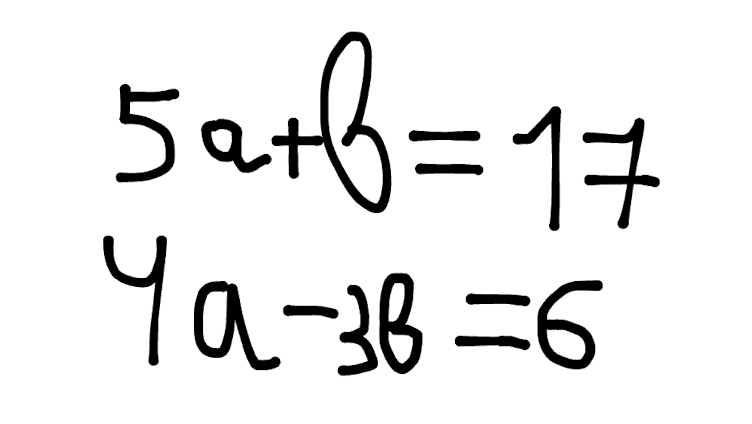
We can do a matrix out of it:

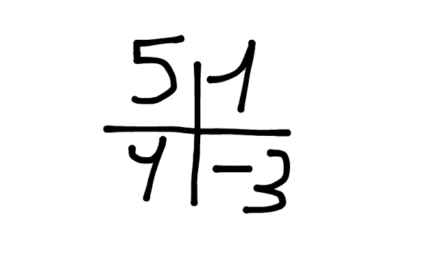
Ok, but why do we need them in Data Science?

They are an important part of this! First of all, many of the stuff used in data science, such as linear regression, or PCA (Principal Component Analysis) involve linear algebra operations that can be efficiently performed using matrices. Sure, it will be “under the hood”, but knowing of basics always comes in handy, especially during debugging.

Moreover, even in the neural networks that are basis of Deep Learning, every neuron is a matrix itself.

What is NumPy?

NumPy is the main package for scientific computing in Python. It performs a wide variety of mathematical operations, one of which is the calculation of matrices.

1 – Basics of NumPy

Before we get started, let’s import NumPy to load its functions.

import numpy as np

Advantages of using NumPy arrays

Arrays are one of the core data structures of the NumPy library, essential for organizing your data. You can think of them as a grid of values, all of the same type. If you have used Python lists before, you may remember that they are convenient, as you can store different data types. However, Python lists are limited in functions and take up more space and time to process than NumPy arrays.

NumPy provides an array object that is much faster and more compact than Python lists. Through its extensive API integration, the library offers many built-in functions that make computing much easier with only a few lines of code. This can be a huge advantage when performing math operations on large datasets.

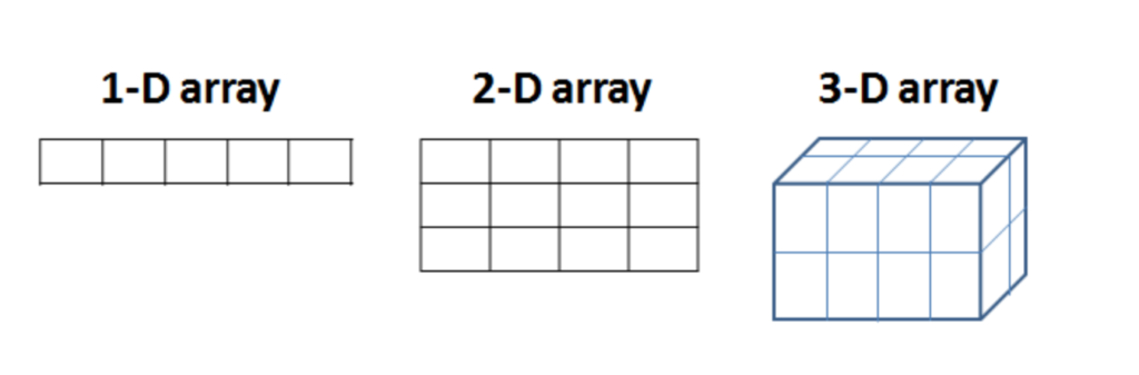
The array object in NumPy is called `ndarray` meaning ‘n-dimensional array’. To begin with, you will use one of the most common array types: the one-dimensional array (‘1-D’). A 1-D array represents a standard list of values entirely in one dimension. Remember that in NumPy, all of the elements within the array are of the same type.

one_dimensional_arr = np.array([10, 12])
print(one_dimensional_arr)

[10, 12]

How to create NumPy arrays

There are several ways to create an array in NumPy. You can create a 1-D array by simply using the function array() which takes in a list of values as an argument and returns a 1-D array.

# Create and print a NumPy array 'a' containing the elements 1, 2, 3.
a = np.array([1, 2, 3])
print(a)

[1, 2, 3]

Another way to implement an array is using np.arange(). This function will return an array of evenly spaced values within a given interval. To learn more about the arguments that this function takes, there is a powerful feature in Jupyter Notebook that allows you to access the documentation of any function by simply pressing shift+tab on your keyboard when clicking on the function. Give it a try for the built-in documentation of np.arange().

# Create an array with 3 integers, starting from the default integer 0.
b = np.arange(3)
print(b)

[0 1 2]

# Create an array that starts from the integer 1, ends at 20, incremented by 3.
c = np.arange(1, 20, 3)
print(c)

[ 1 4 7 10 13 16 19]

What if you wanted to create an array with five evenly spaced values in the interval from 0 to 100? As you may notice, you have 3 parameters that a function must take. One paremeter is the starting number, in this case 0, the final number 100 and the number of elements in the array, in this case, 5. NumPy has a function that allows you to do specifically this by using np.linspace().

lin_spaced_arr = np.linspace(0, 100, 5)
print(lin_spaced_arr)

[ 0. 25. 50. 75. 100.]

Did you notice that the output of the function is presented in the float value form (e.g. “… 25. 50. …”)? The reason is that the default type for values in the NumPy function np.linspace is a floating point (np.float64). You can easily specify your data type using dtype. If you access the built-in documentation of the functions, you may notice that most functions take in an optional parameter dtype. In addition to float, NumPy has several other data types such as int, and char.

To change the type to integers, you need to set the dtype to int. You can do so, even in the previous functions. Feel free to try it out and modify the cells to output your desired data type.

lin_spaced_arr_int = np.linspace(0, 100, 5, dtype=int)
print(lin_spaced_arr_int)

[ 0 25 50 75 100]

c_int = np.arange(1, 30, 4, dtype=int)
print(c_int)

[ 1 5 9 13 17 21 25 29]

b_float = np.arange(3, dtype=float)
print(b_float)

[0. 1. 2.]

More on NumPy arrays

One of the advantages of using NumPy is that you can easily create arrays with built-in functions such as:

np.ones() – Returns a new array setting values to one.
np.zeros() – Returns a new array setting values to zero.
np.empty() – Returns a new uninitialized array.
np.random.rand() – Returns a new array with values chosen at random.

# Return a new array of shape 3, filled with ones. 
ones_arr = np.ones(3)
print(ones_arr)

[1. 1. 1.]

# Return a new array of shape 3, filled with zeroes. 
zeros_arr = np.zeros(3)
print(zeros_arr)

[0. 0. 0.]

# Return a new array of shape 3, without initializing entries.
empt_arr = np.empty(3)
print(empt_arr)

[0. 0. 0.]

# Return a new array of shape 3 with random numbers between 0 and 1.
rand_arr = np.random.rand(3)
print(rand_arr)

[0.45608517 0.33116721 0.30509029]

2 – Multidimensional Arrays

With NumPy you can also create arrays with more than one dimension. In the above examples, you dealt with 1-D arrays, where you can access their elements using a single index. A multidimensional array has more than one column. Think of a multidimensional array as an excel sheet where each row/column represents a dimension.

# Create a 2 dimensional array (2-D)
two_dim_arr = np.array([[1,2,3], [4,5,6]])
print(two_dim_arr)

[[1 2 3]

[4 5 6]]

An alternative way to create a multidimensional array is by reshaping the initial 1-D array. Using np.reshape() you can rearrange elements of the previous array into a new shape.

#1-D array
one_dim_arr = np.array([1, 2, 3, 4, 5, 6])

# Multidimensional array using reshape()
multi_dim_arr = np.reshape(
                        one_dim_arr, # the array to be reshaped
                        (2,3) # dimensions of the new array
                       )

# Print the new 2-D array with two rows and three columns
print(multi_dim_arr)

Finding size, shape and dimension.

In future assignments, you will need to know how to find the size, dimension and shape of an array. These are all atrributes of a ndarray and can be accessed as follows:

ndarray.ndim – Stores the number dimensions of the array.
ndarray.shape – Stores the shape of the array. Each number in the tuple denotes the lengths of each corresponding dimension.
ndarray.size – Stores the number of elements in the array.

# Dimension of the 2-D array multi_dim_arr
multi_dim_arr.ndim

# Shape of the 2-D array multi_dim_arr
# Returns shape of 2 rows and 3 columns
multi_dim_arr.shape

(2, 3)

# Size of the array multi_dim_arr
# Returns total number of elements
multi_dim_arr.size

3 – Array math operations

In this section, you will see that NumPy allows you to quickly perform elementwise addition, substraction, multiplication and division for both 1-D and multidimensional arrays. The operations are performed using the math symbol for each ‘+’, ‘-‘ and ‘*’. Recall that addition of Python lists works completely differently as it would append the lists, thus making a longer list, in addition, subtraction and multiplication of Python lists do not work.

arr_1 = np.array([2, 4, 6])
arr_2 = np.array([1, 3, 5])

# Adding two 1-D arrays
addition = arr_1 + arr_2
print(addition)

# Subtracting two 1-D arrays
subtraction = arr_1 - arr_2
print(subtraction)

# Multiplying two 1-D arrays elementwise
multiplication = arr_1 * arr_2
print(multiplication)

[ 3 7 11]

[1 1 1]

[ 2 12 30]

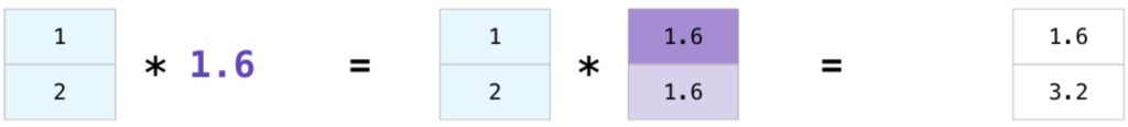
Multiplying vector with a scalar (broadcasting)

Suppose you need to convert miles to kilometers. To do so, you can use the NumPy array functions that you’ve learned so far. You can do this by carrying out an operation between an array (miles) and a single number (the conversion rate which is a scalar). Since, 1 mile = 1.6 km, NumPy computes each multiplication within each cell.

This concept is called broadcasting, which allows you to perform operations specifically on arrays of different shapes.

vector = np.array([1, 2])
vector * 1.6

array([1.6, 3.2])

4 – Indexing and slicing

Indexing is very useful as it allows you to select specific elements from an array. It also lets you select entire rows/columns or planes as you’ll see in future assignments for multidimensional arrays.

4.1 – Indexing

Let us select specific elements from the arrays as given.

# Select the third element of the array. Remember the counting starts from 0.
a = ([1, 2, 3, 4, 5])
print(a[2])

# Select the first element of the array.
print(a[0])

For multidimensional arrays of shape n, to index a specific element, you must input n indices, one for each dimension.

# Indexing on a 2-D array
two_dim = np.array(([1, 2, 3],
          [4, 5, 6], 
          [7, 8, 9]))

# Select element number 8 from the 2-D array using indices i, j.
# 3rd row and 2nd column
print(two_dim[2][1])

4.2 – Slicing

Slicing gives you a sublist of elements that you specify from the array. The slice notation specifies a start and end value, and copies the list from start up to but not including the end (end-exclusive).

The syntax is:

array[start:end:step]

If no value is passed to start, it is assumed start = 0, if no value is passed to end, it is assumed that end = length of array - 1 and if no value is passed to step, it is assumed step = 1.

# Slice the array a to get the array [2,3,4]
sliced_arr = a[1:4]
print(sliced_arr)

[2, 3, 4]

# Slice the array a to get the array [3,4,5]
sliced_arr = a[2:]
print(sliced_arr)

# Slice the array a to get the array [1,3,5]
sliced_arr = a[::2] # default start index, default stop index, step size is two—take every second element
print(sliced_arr)

# Note that a == a[:] == a[::]
print(a == a[:] == a[::])

True

# Slice the two_dim array to get the first two rows
sliced_arr_1 = two_dim[0:2]
sliced_arr_1

array([[1, 2, 3],

[4, 5, 6]])

# Similarily, slice the two_dim array to get the last two rows
sliced_two_dim_rows = two_dim[1:3]
print(sliced_two_dim_rows)

[[4 5 6]

[7 8 9]]

sliced_two_dim_cols = two_dim[:,1]
print(sliced_two_dim_cols)

[2 5 8]

5 – Stacking

Finally, stacking is a feature of NumPy that leads to increased customization of arrays. It means to join two or more arrays, either horizontally or vertically, meaning that it is done along a new axis.

np.vstack() – stacks vertically
np.hstack() – stacks horizontally
np.hsplit() – splits an array into several smaller arrays

a1 = np.array([[1,1], 
               [2,2]])
a2 = np.array([[3,3],
              [4,4]])
print(f'a1:\n{a1}')
print(f'a2:\n{a2}')

a1:

[[1 1]

[2 2]]

a2:

[[3 3]

[4 4]]

# Stack the arrays vertically
vert_stack = np.vstack((a1, a2))
print(vert_stack)