Feature engineering
Machine learning is not just about picking the right parameters for a model. ML workflows depend on feature engineering and selection. In many Data Science communities these concepts are mistakenly equated. Let’s understand why we need features, and explore the peculiarities of implementing feature engineering techniques.
What are features and what they are?
A feature is a variable (a column in a table) that describes a particular characteristic of an object. Features are the cornerstone of machine learning tasks in general; they are the basis on which we build predictions in models.
Features can be of the following types:
- Binary, which take only two values. For example, [true, false], [0,1], [“yes”, “no”].
- Categorical (or nominal). They have a finite number of levels, for example the attribute “day of the week” has 7 levels: Monday, Tuesday, etc., until Sunday.
- Arranged. These are somewhat similar to categorical signs. The difference between them is that in this case there is a clear ordering of categories. For example, “grades in school” from 1 to 12. This can also include “time of day”. which has 24 levels and is ordered.
- Numerical (quantitative). These are values ranging from minus infinity to plus infinity, which cannot be attributed to the previous three types of features.
Note that for machine learning tasks, we need only those “features” that actually affect the final result are needed.
What is Feature Engineering?
Feature Engineering is the process by which we extract new variables for a table from raw data. In life, data rarely comes in the form of ready-made matrices, so any task starts with feature extraction.
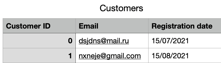
For example, an online shop’s database has a table called “Customers”, which contains one row for each customer who visited the site.
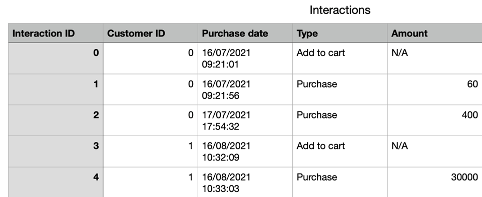
It can also have an “Interactions” table that contains a row for each interaction (click or page visit) that the customer made on the site. This table also contains information about the time of the interaction and the type of event that represented the interaction (a “Purchase”, “Search” or the “Add to cart” event ). These two tables are linked with the Customer ID column.
To predict when a customer will buy an item next time, we would like to get a single numerical attribute matrix with a row for each customer. We can then use this in a machine learning algorithm. However, the table that most closely resembles this (“Shoppers”) contains almost no relevant information. We can build some characteristics from it, such as the number of days since a customer registered, but our ability at this stage is limited.
To increase our predictive power score (PPS), we must use the data in the interaction table. Feature selection makes this possible. We can calculate statistics for each client using all the values in the Interactions table with that client’s ID. Here are some potentially useful traits or “features” to help us solve the problem:
• Average time between past purchases.
• Average amount of that.
• The maximum amount of past purchases.
• Time had elapsed since last acquisition.
• The total number of past purchases.
To build these attributes, we must find all the interactions associated with a particular client. Then we will filter those whose Type is not “Purchase” and calculate a function that returns a single value using the available data.
Note that this process is unique to each use case and dataset.
This type of feature engineering is necessary for effective use of machine learning algorithms and predictive model building.
The main and best known feature engineering methods will be listed below, with a brief description and implementation code.
Build features on tabular data.
Removal of missing values.
Missing values are one of the most common problems you may encounter when trying to prepare data. This factor greatly affects the performance of machine learning models.
The simplest solution for missing values is to discard rows or an entire column. There is no optimal threshold for discarding, but you can use 70% as the value and discard rows with columns missing values that exceed this threshold.
import pandas as pd
import numpy as np
threshold = 0.7
# Removing columns with a missing value ratio above the threshold
data = data[data.columns[data.isnull().mean() < threshold]]
# Remove rows with no-value ratio above the threshold
data = data.loc[data.isnull().mean(axis=1) < threshold]
Filling in the missing values.
This is preferable to discarding because it preserves the size of the data. It is very important what exactly you attribute to the missing values. For instance, if you have a column with the numbers 1 and N/A , it is likely that the rows N/A correspond to 0.
As another example, you have a column that shows the number of customer visits in the last month. This is where the missing values can be replaced with 0.
With the exception of the above, the best way to fill in the missing values is to use medians of all columns. As column averages are sensitive to outlier values, medians will be more robust in this respect.
import pandas as pd
import numpy as np
# Filling all missing values 0
 data = data.fillna (0)
# Filling the missing values with the medians of the columns
 data = data.fillna (data.median ())
Replacing missing values with maximum values.
Replacing missing values with the maximum value in the column would only be a good option to work with when dealing with categorical features. In other situations, the previous method is highly recommended.
import pandas as pd
import numpy as np
data['column_name'].fillna(data['column_name'].value_counts() .idxmax
(), inplace=True)
Detecting outliers.
Before I mention how outliers can be handled, I want to state that the best way to detect outliers is to perform a visualisation of your dataset. The libraries seaborn and matplotlib can help you with this.
For detecting outliers: one of the best ways to do this is to calculate the standard deviation. If a value deviates by more than x * standard deviation , it can be taken as an outlier. The most used value for x is within [2, 4].
import pandas as pd
import numpy as np
# Removing unappropriate rows
x = 3
upper_lim = data['column'].mean () + data['column'].std () * x lower_lim = data['column'].mean () - data['column'].std () * x
data = data[(data['column'] < upper_lim) & (data['column'] > lower_li m)]
Another mathematical method of detecting emissions is to use percentiles. You take a certain percentage of the value at the top or bottom as an outlier.
The key here is to re-set the percentile value, and this depends on the distribution of your data, as mentioned earlier.
Moreover, a common mistake is to use percentiles according to the range of your data. In other words, if your data is between 0 and 100 , your top 5% are not values between 96 and 100 . The top 5% refers here to values outside the 95th percentile of the data.
import pandas as pd
import numpy as np
# Get rid of unnecessary rows by using percentiles
upper_lim = data['column'].quantile(.95)
lower_lim = data['column'].quantile(.05)
data = data[(data['column'] < upper_lim) & (data['column'] > lower_li
m)]
Limit emissions.
Another option for handling outliers is to limit them rather than discard them. You will be able to maintain your data size, and this may be better for the final performance of the model.
On the other hand, limiting can affect the distribution of the data and the quality of the model, so it is better to stick to the golden mean.
import pandas as pd
import numpy as np
upper_lim = data['column'].quantile(.95)
lower_lim = data['column'].quantile(.05)
data.loc[(df[column] > upper_lim),column] = upper_lim
data.loc[(df[column] < lower_lim),column] = lower_lim
The logarithmic transformation.
The logarithmic transformation is one of the most common mathematical transforms used during feature engineering.
- It helps to handle distorted data, and after the transformation, the distribution becomes closer to normal.
- In most cases, the order of magnitude of the data varies within the range of the data. For example, a difference between 15 and 20 years of age does not equal a difference between 65 and 70 years of age, as in all other aspects a difference of 5 years at a young age means a larger difference in magnitude. This type of data comes from a multiplicative process, and the logarithmic transformation normalises such differences in magnitudes.
• It also reduces the impact of outliers by normalising the difference in values, and the model becomes more robust.
Important note: the data you apply must only have positive values, otherwise you will get an error.
import pandas as pd
import numpy as np
# An exaple of logarithmic transformation
data = pd.DataFrame({'value':[2,45, -23, 85, 28, 2, 35, -12]})
data['log+1'] = (data['value']+1).transform(np.log)
# Handling negative values
# (Note that the values are different)
data['log'] = (data['value']-data['value'].min()+1) .transform(np.log
)
One-Hot encoding.
This method distributes the values in a column over multiple flag columns and assigns
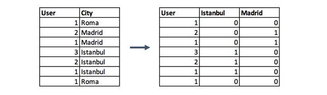
them 0 or 1. Binary values represent the relationship between the grouped column and the
encoded column. This method changes your categorical data into a numerical format, which is difficult for algorithms to understand. The grouping is done without losing any information, for example:
The below function reflects the use of the fast coding method with your data.
encoded_columns = pd.get_dummies(data['column'])
data = data.join(encoded_columns).drop('column', axis=1)
Feature scaling.
In most cases, the numerical characteristics of a dataset do not have a defined range and differ from each other.
For example, the age and monthly wage columns will have completely different ranges.
How can these two columns be compared if this is necessary in our task? Scaling solves this problem, because after this operation the items become identical in range.
There are two common ways of scaling:
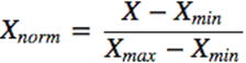
- Normalisation.
In this case, all values will be in the range 0 to 1. Discrete binary values are defined as 0 and 1.
import pandas as pd
import numpy as np
data = pd.DataFrame({'value':[2,45, -23, 85, 28, 2, 35, -12]})
data['normalized'] = (data['value'] - data['value'].min()) / (data['v
alue'].max() - data['value'].min()) - Standardisation.
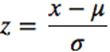
It scales the values to account for the standard deviation. If the standard deviation of the functions is different, their range will also be different from each other. This reduces the effect of outliers in the elements. In the following standardisation formula, the mean value is shown as μ and the standard deviation is shown as σ.
import pandas as pd
import numpy as np
data = pd.DataFrame({'value':[2,45, -23, 85, 28, 2, 35, -12]})
data['standardized'] = (data['value'] - data['value'].mean()) / data[
'value'].std()
Working with text.
There are too many methods of working with text to fit into one thesis statement. Nevertheless, the most popular approach will be described below.
Before working with text, it must be broken down into tokens – individual words. However, by doing this too simply, we may lose some of the meaning. For example, “New York” is not two tokens, but one.
After turning the document into a sequence of words, we can start turning them into vectors. The simplest method is Bag of Words. We create a vector of length in the dictionary, for each word we count the number of occurrences in the text and substitute this number for the corresponding position in the vector.
In code, the algorithm looks much simpler than in words:
from functools import reduce
import numpy as np
texts = [['i', 'have', 'a', 'cat'],
         ['he', 'have', 'a', 'dog'],
         ['he', 'and', 'i', 'have', 'a', 'cat', 'and', 'a', 'dog']]
dictionary = list(enumerate(set(reduce(lambda x, y: x + y, texts))))
def vectorize(text):
    vector = np.zeros(len(dictionary))
    for i, word in dictionary:
        num = 0
        for w in text:
            if w == word:
Working with images.
As far as images are concerned, methods of constructing and extracting features for this type of data are among the simplest.
Often a particular convolutional network is used for image tasks. It is not necessary to design the network architecture and train it from scratch. It is possible to borrow an already trained neural network from the open source.
To adapt it to their task, data scientists practice fine tuning. The last layers of the neural network are removed, new layers are added instead, tailored to our specific task, and the network is retrained on the new data.
An example of this pattern:
from keras.applications.resnet50 import ResNet50
from keras.preprocessing import image
from scipy.misc import face
import numpy as np
resnet_settings = {'include_top': False, 'weights': 'imagenet'}
resnet = ResNet50(**resnet_settings)
img = image.array_to_img(face())
img = img.resize((224, 224))
# you may need to be more careful about resizing
x = image.img_to_array(img)
x = np.expand_dims(x, axis=0)
# extra dimensioning is needed, as the model is designed to work with an image array
features = resnet.predict(x)
Conclusion.
Correct feature construction is essential in improving our machine learning models. Without this step, we cannot implement the subsequent feature selection technique.
In practice, the process of feature construction can be varied. Solving the problem of missing values, detecting outliers, turning text into a vector (using advanced NLP which embed words into vector space) are just a few examples from this area.
The next article will focus on Featire Selection.