The k Nearest Neighbors (kNN) method is a popular classification algorithm that is used in various types of machine learning tasks. Along with the decision tree, it is one of the most comprehensible approaches to classification.
What’s that?
On an intuitive level, the essence of the method is simple: look at the neighbours around you, which ones prevail, that’s what you are. Formally the basis of the method is the compactness hypothesis: if the metric of distance between examples is introduced successfully, similar examples are much more likely to lie in the same class than in different ones.
- If the method is used for classification, the object is assigned to the class that is most common among the k neighbours of the given item whose classes are already known.
- If the method is used for regression, the object is assigned to the average of the k nearest objects whose values are already known.
An example of k nearest neighbour classification.
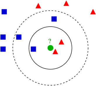
- We have a test pattern in the form of a green circle. We will label the blue squares as class 1, the red triangles as class 2.
- The green circle must be classified as class 1 or class 2. If the area we are considering is a small circle, the object is classified as class 2 because there are 2 triangles and only 1 square inside this circle.
- If we are considering a large circle (with a dotted line), the circle will be classified as class 1 because there are 3 squares inside the circle as opposed to 2 triangles.
The theoretical component of the k-NN algorithm
Beyond a simple explanation, it is necessary to understand the basic mathematical components of the k-nearest neighbour algorithm.
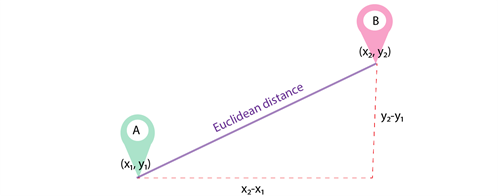
The Euclidean metric (Euclidean distance) is a metric in Euclidean space, the distance between two points in Euclidean space calculated by Pythagoras’ theorem. Simply put, it is the shortest possible distance between points A and B. Although the Euclidean distance is useful for small dimensions, it does not work for large dimensions and for categorical variables. A disadvantage of the Euclidean distance is that it ignores the similarity between attributes. Each of them is treated as completely different from all the others.
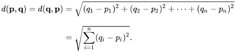
The formula for calculating the Euclidean distance:
- Another important component of the method is normalization. Different attributes usually have different ranges of represented values in the sample. For example, attribute A is represented in the range 0.01 to 0.05, while attribute B is represented in the range 500 to 1000). In this case, distance values can be highly dependent on attributes with larger ranges. Therefore, the data in most cases go through normalisation. In cluster analysis there are two main ways to normalize data: MinMax-normalization and Z-normalization.
MinMax normalization is carried out as follows:
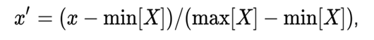
In this case, all values will be in the range 0 to 1; discrete binary values are defined as 0 and 1.
Z-normalization:
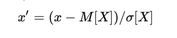
Where σ is the standard deviation. In this case most of the values
fall within the range.
What is the procedure?
- Load your data.
- Initialise k by selecting the optimal number of neighbours.
- For each sample in the data:
- Calculate the distance between the query sample and the current sample in the data.
- Add the index of the sample to the ordered collection, like its distance.
- Sort the ordered collection of distances and indices from smallest to largest, in ascending order.
- Select the first k records from the sorted collection.
- Take the labels of the selected k records.
- If you have a regression problem, return the average of the previously selected k labels.
- If you have a classification problem, return the most frequent value of the previously chosen k labels.
Python implementation
For the demonstration we will use the most common sandbox competition in Kaggle: Titanic. You can find the data here. We aim to use the python library for machine learning scikit-learn. We use the Titanic dataset for logistic regression.
The dataset consists of 15 columns, such as sex (gender), fare, p_class (cabin class), family_size, etc. The main attribute that we have to predict in the competition is whether or not the passenger survived.
Additional analysis showed that married people have a higher chance of being rescued from the ship. Therefore 4 more columns were added, renamed from Name, to denote men and women according to whether they were married or not (Mr, Mrs, Mister, Miss).
The full dataset can be downloaded from here and the full code for this article can be found here.
To clearly demonstrate the functionality of k-NN for predicting passenger survival, we consider only two features: age, fare.
# Load the data
train_df = pd.read_csv('/kaggle/input/titanic/train_data.csv')
# Remove 2 columns with unnecessary information
train_df = train_df.drop(columns=['Unnamed: 0', 'PassengerId'])
from sklearn.neighbors import KNeighborsClassifier
predictors = ['Age', 'Fare']
outcome = 'Survived'
new_record = train_df.loc[0:0, predictors]
X = train_df.loc[1:, predictors]
y = train_df.loc[1:, outcome]
kNN = KNeighborsClassifier(n_neighbors=20)
kNN.fit(X, y)
kNN.predict(new_record)
Here, the probability of survival is 0.3 – 30%.
Next, we set up the k-NN algorithm to find and use the 20 nearest neighbours to estimate the passenger’s condition. For clarity, we output the 20 first neighbours of the new record using the imported kneighbors method. The implementation looks as follows:
nbrs = knn.kneighbors(new_record)
maxDistance = np.max(nbrs[0][0])
fig, ax = plt.subplots(figsize=(10, 8))
sns.scatterplot(x = 'Age', y = 'Fare', style = 'Survived',
                hue='Survived', data=train_df, alpha=0.3, ax=ax)
sns.scatterplot(x = 'Age', y = 'Fare', style = 'Survived',
                hue = 'Survived',
                data = pd.concat([train_df.loc[0:0, :], train_df.loc[
nbrs[1][0] + 1,:]]),
                ax = ax, legend=False)
ellipse = Ellipse(xy = new_record.values[0],
                  width = 2 * maxDistance, height = 2 * maxDistance,
                  edgecolor = 'black', fc = 'None', lw = 1)
ax.add_patch(ellipse)
The result of the code:
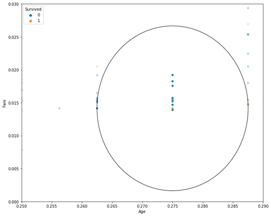
As you can see, the graph shows 20 nearest neighbours, 14 of which are related to survivors (probability 0.7 – 70%), and 6 are related to survivors (probability 0.3 – 30%).
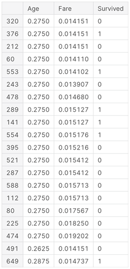
We can look up the first 20 nearest neighbours for the given parameters using the following code:
nbrs = knn.kneighbors(new_record)
nbr_df = pd.DataFrame({'Age': X.iloc[nbrs[1][0], 0],
'Fare': X.iloc[nbrs[1][0], 1],
'Survived': y.iloc[nbrs[1][0]]})
nbr_df
The result will be:
Choosing the Optimal value for k-NN
There is no particular way to determine the best value for k, so we need to try several values to find the best one. But most often the most preferred value for k is 5:
- A low value of k, such as 1 or 2, can lead to an under-learning effect on the model.
- A high value of k seems acceptable at first glance, but there may be difficulties with model performance, and there is an increased risk of overtraining.
Advantages and disadvantages
Advantages:
- The algorithm is simple and easy to implement.
- It is not sensitive to emissions.
- There is no need to build a model, adjust multiple parameters or make additional assumptions.
- The algorithm is versatile. It can be used for both types of tasks: classification and regression.
Disadvantages:
- The algorithm is significantly slower when the sample size, predictors or independent variables are increased.
- From the argument above, there are high computational costs at runtime.
- It is always necessary to determine the optimal value of k.
In conclusion
The k-nearest neighbours method is a simple machine learning algorithm with a teacher that can be used for classification and regression problems. It is easy to implement and understand, but has the significant disadvantage of being significantly slower when the amount of data grows.
The algorithm finds distances between a query and all examples in the data, selects a certain number of examples (k) closest to the query, then votes for the most frequent label (in the case of the classification problem) or averages the labels (in the case of the regression problem).